Full text search:
Home > Abstract >Physics
Introduction……………………………………………………………..... 3
Flow of tension electric field. Gauss's theorem in integral form……………………………………………………4
The emergence and development of the theory of the electromagnetic field……….. 8
Conclusion ……………………………………………………………. 15
List of used literature………………………………. 16
Introduction
According to modern ideas, electric charges do not act on each other directly. Each charged body creates an electric field in the surrounding space, which exerts a force on other charged bodies.
The main property of the electric field is the effect on electric charges with some force. Thus, the interaction of charged bodies is carried out not by their direct influence on each other, but through the electric fields surrounding the charged bodies.
To quantitatively determine the electric field, a force characteristic is introduced - the electric field strength.
Electric field strength is a physical quantity equal to the ratio of the force with which the field acts on a positive test charge placed at a given point in space to the magnitude of this charge:
Electric field strength is a vector physical quantity. The direction of the vector E coincides at each point in space with the direction of the force acting on the positive test charge.
The electric field strength created by a system of charges at a given point in space is equal to the vector sum of the electric field strengths created at the same point by charges separately:
![]()
This property of the electric field means that the field obeys the principle of superposition.
Electric field strength flow. Gauss's theorem in integral form
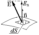
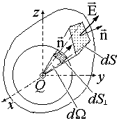
Let n be the unit normal to the area dS (small enough to neglect the change in electrical intensity E within the area). The flow dФ e of electrical intensity through this area is defined as the product of the normal component E and dS:
The sign of the flux dF e obviously depends on the relative orientation of the normal and the tension. If these two vectors form an acute angle, the flux is positive; if it is obtuse, the flux is negative.
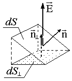
The flux dF e through an area inclined to the line of force (i.e., to vector E) is also equal to the flux through the projection of this area onto a plane perpendicular to the line of force (see Fig. 1.1.2):
This equality (1.1.1) follows from the definition (1.1.1) for dF e and the theorem on angles with mutually perpendicular sides.
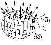
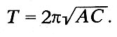
The flow F e of electrical intensity E through a closed surface S (Fig. 1.3.3) is defined as the sum of elementary flows through all areas of the surface. In the limit, when the number of sites N tends to infinity, the sum of the fluxes through the sites goes into the surface integral of the normal component of tension E n:
In 1844, K. Gauss proved a theorem (Gauss's theorem in integral form) establishing the connection between field sources and intensity flow through an arbitrary surface surrounding the sources.
![]()
To prove this, we derive an auxiliary formula. Stream from point charge through an arbitrary sphere surrounding it.
 .
(1.1.4)
.
(1.1.4)
The field lines of a point charge are perpendicular to the surface of a concentric sphere (see Fig. 1.1.4). Taking this fact into account, formula (1.1.4) is derived from the expression for the field of a point charge. As can be seen, in this case the flow F e does not depend on the radius of the sphere, but depends only on Q.
From (1.1.2) and (1.1.4) it follows that the field flux of a point charge through any surface surrounding the charge is equal to the flux through a sphere of arbitrary radius concentric to the charge. Indeed, the flow of the field of a point charge through any area dS cut by a solid angle d from an arbitrary surface is the same as the flow through an area of a sphere cut by the same solid angle. The field flow F e through the sphere, as already noted, does not depend on its radius. Therefore, the field strength flux of a point charge through the surface S (see Fig. 1.3.5) is given by formula (1.3.4). From formula (1.3.4) and the principle of superposition follows the Gauss theorem in integral form: the total flux F e of the electric field strength through an arbitrary closed surface, inside which there is an arbitrarily distributed (volume, surface, etc.) charge Q, is calculated by formula
When applying Gauss's theorem to solve problems, it is necessary to remember that in equation (1.1.5) Q is the sum of all charges inside the mental surface through which the flux is calculated, including charges belonging to atoms and molecules of the medium (the so-called bound charges).
The flux of field strength E through any closed surface within which there is a total charge equal to zero, is also zero.
The emergence and development of the theory of electromagnetic field
In the 17th and 18th centuries, electromagnetic processes penetrated deeper and deeper into science: physics and chemistry. The era of the electromagnetic picture of the world was coming, replacing the mechanical one.
Maxwell clearly saw the fundamental importance of electromagnetic laws, carrying out a grand synthesis of optics and electricity. It was he who managed to reduce optics to electromagnetism, creating the electromagnetic theory of light and thereby paving new paths not only in theoretical physics, but also in technology, preparing the ground for radio engineering.
Faraday took a new approach to the study of electricity and magnetic phenomena, indicating the role of the environment and introducing the concept of the field described by it using power lines. Maxwell gave the ideas mathematical completeness, introduced the precise term “electromagnetic field,” which Faraday did not yet have, and formulated the mathematical laws of this field. Galileo and Newton laid the foundations mechanical picture world, Faraday and Maxwell - the foundations of the electromagnetic picture of the world.
Maxwell developed electromagnetic theory in his works “On Physical Lines of Force” (1861-1862) and “Dynamic Field Theory” (1864-1865). He wrote these works no longer in Aberdeen, but in London, where he received a professorship at King's College. Here Maxwell met with Faraday, who was already old and sick. Maxwell, having received data confirming the electromagnetic nature of light, sent them to Faraday. Maxwell wrote: “The electromagnetic theory of light, proposed by him (Faraday) in “Thoughts on Ray Vibrations” (Phil. Mag., May 1846) or “Experimental Investigations” (Exp. Rec., p. 447), is essentially that the same as what I began to develop in this article ("Dynamic Field Theory" - Phil. Mag., 1865), except that in 1846 there was no data to calculate the speed of propagation. J.K.M.”
In 1873, Maxwell's main work, “Treatise on Electricity and Magnetism,” was published. He began writing a popular exposition of his theory, “Electricity in Elementary Exposition,” but did not have time to finish it.
Maxwell was a versatile scientist: theorist, experimenter, and technician. But in the history of physics, his name is primarily associated with the theory of the electromagnetic field he created, which is called Maxwell’s theory or Maxwellian electrodynamics. It entered the history of science along with such fundamental generalizations as Newtonian mechanics, relativistic mechanics, quantum mechanics, and marked the beginning of a new stage in physics. In accordance with the law of the development of science, formulated by Aristotle, it raised the knowledge of nature to a new, higher level and at the same time was more incomprehensible, abstract than previous theories, “less obvious to us,” as Aristotle put it.
Maxwell began developing his theory in 1854.
Maxwell characterizes the electrotonic state with the help of three functions, which he calls electrotonic functions or components of the electrotonic state. In modern notation, this vector function corresponds to the vector potential. The line integral of this vector along a closed line is what Maxwell calls the “total electrotonic intensity along a closed curve.” For this quantity, he finds the first law of the electrotonic state: “The total electrotonic intensity along the boundary of a surface element serves as a measure of the amount of magnetic induction passing through that element, or, in other words, as a measure of the number of magnetic lines of force penetrating a given element.” In modern notation, this law can be expressed by the formula:
where A is the component of the potential vector in the direction of the curve element dl, Bn ~ the normal component of the induction vector B in the direction of the normal to the surface element dS.
connecting magnetic induction B with the voltage vector magnetic field N.
The third law relates the magnetic field strength H to the strength of the current I creating it. Maxwell formulates it this way: “The total magnetic intensity along a line delimiting any part of a surface serves as a measure of the amount of electric current flowing through that surface.” In modern notation, this sentence is described by the formula
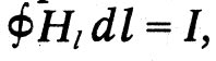
which is now called Maxwell's first equation in integral form. It reflects the experimental fact discovered by Oersted: the current is surrounded by a magnetic field.
The fourth law is Ohm's law:
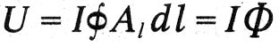
To characterize the force interactions of currents, Maxwell introduces a quantity he calls magnetic potential. This quantity obeys the fifth law: “The total electromagnetic potential of a closed current is measured by the product of the amount of current and the total electrotonic intensity along the circuit, calculated in the direction of the current:
Maxwell's sixth law applies to electromagnetic induction: "The electromotive force acting on a conductor element is measured by the time derivative of the electrotonic intensity, whether that derivative is due to a change in the magnitude or direction of the electrotonic state." In modern notation, this law is expressed by the formula:

This is Maxwell's second equation in integral form. Note that Maxwell refers to the circulation of the electric field strength vector as electromotive force. Maxwell generalizes the Faraday-Lenz-Neumann law of induction, considering that a change in time of a magnetic flux (electrotonic state) generates a vortex electric field that exists regardless of whether there are closed conductors in which this field excites a current or not. Maxwell has not yet given a generalization of Oersted's law.
Another important news is the introduction of the concepts of bias and bias currents. Displacement, according to Maxwell, is a characteristic of the states of a dielectric in an electric field. The total displacement flux through a closed surface is equal to the algebraic sum of the charges located inside the surface. This introduces the fundamental concept of displacement current. This current, like the conduction current, creates a magnetic field. Therefore, Maxwell generalizes the equation, which is now called Maxwell's first equation, and introduces a displacement current into the first part. In modern notation, this Maxwell equation has the form:
![]()
And finally, Maxwell finds that transverse waves propagate in his elastic medium at the speed of light. This fundamental result leads him to an important conclusion: “The speed of transverse wave oscillations in our hypothetical medium, calculated from the electromagnetic experiments of Kohlrausch and Weber, coincides so exactly with the speed of light calculated from the optical experiments of physics that we can hardly refuse the conclusion that light consists of transverse vibrations of the same medium that causes electrical and magnetic phenomena. Thus, in the early 60s of the XIX century. Maxwell had already found the basis of his theory of electricity and magnetism and made the important conclusion that light is an electromagnetic phenomenon.
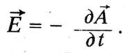
In Maxwell's theory, the quantity "electromagnetic torque" is related to magnetic flux. The circulation of the potential vector along a closed loop is equal to the magnetic flux through the surface covered by the loop. Magnetic flux has inertial properties, and the electromotive force of induction according to Lenz's rule is proportional to the rate of change of the magnetic flux, taken with the opposite sign. Hence the intensity of the induction electric field:
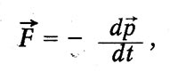
Maxwell considers this expression to be similar to the expression for the force of inertia in mechanics:
![]()
Mechanical impulse, or momentum. This analogy explains the term introduced by Maxwell for the vector potential. The electromagnetic field equations themselves in Maxwell's theory have a form different from the modern one.
In its modern form, Maxwell's system of equations has the following form:
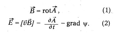
The relationship between the displacement vector D and the electric field strength E in Maxwell is expressed by the equation:
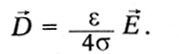
![]()
Then writes out the equation divD = p and the equation where
![]()
and also the boundary condition:
![]()
This is Maxwell's system of equations. The most important conclusion from these equations is the existence of transverse electromagnetic waves propagating in a magnetized dielectric with speed: where
![]()
He obtained this conclusion in the last section of “Dynamic Field Theory,” called “Electromagnetic Theory of Light.” “...The science of electromagnetism,” Maxwell writes here, “leads to exactly the same conclusions as optics regarding the direction of disturbances that can propagate through a field; both of these sciences affirm the transversality of these vibrations, and both give the same speed of propagation.” In the ether, this speed c is the speed of light (Maxwell denotes it V), in a dielectric it is less where
Thus, the refractive index n, according to Maxwell, is determined by the electrical and magnetic properties of the medium. In a non-magnetic dielectric where
![]()
This is Maxwell's famous relation.
In 1853, V. Thomson investigated the discharge of a conductor of a given capacity through a conductor of a given shape and resistance. Applying the law of conservation of energy to the discharge process, he derived the discharge process equation in the following form:
where q is the amount of electricity on the discharged conductor at a given time t, C is the capacitance of the conductor, k is the galvanic resistance of the spark gap, A is “a constant that can be called the electrodynamic capacitance of the spark gap” and which we now call the self-inductance coefficient or inductance. Thomson, analyzing the solution of this equation for various roots of the characteristic equation, finds that when the quantity
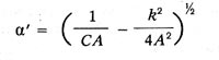
has a real value (1/CA>4*(k/A)2), then the solution shows “that the main conductor loses its charge, is charged with a smaller amount of electricity of the opposite sign, is discharged again, and again finds itself charged with an even smaller amount of electricity of the original sign, and this phenomenon is repeated an infinite number of times until equilibrium is established.” The cyclic frequency of these damped oscillations is:
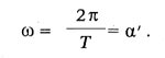
Thus, the oscillation period can be represented by the formula:
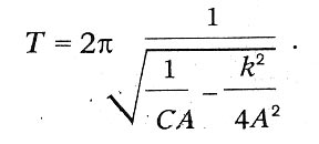
At low resistance values we obtain the well-known Thomson formula:
Conclusion
An electric field is a special form of field that exists around bodies or particles with an electric charge, as well as in free form in electromagnetic waves. The electric field is directly invisible, but can be observed by its action and with the help of instruments. The main effect of the electric field is the acceleration of bodies or particles with an electric charge.
The electric field can be considered as a mathematical model that describes the value of the electric field strength at a given point in space. Douglas Giancoli wrote: “It should be emphasized that the field is not some kind of substance; it is more correct to say that it is an extremely useful concept ... The question of the “reality” and existence of the electric field is in fact a philosophical, rather even metaphysical question. In physics, the idea of The field has proven to be extremely useful - it is one of the greatest achievements of the human mind."
The electric field is one of the components of a single electromagnetic field and a manifestation of electromagnetic interaction.
List of used literature
Dmitrieva V.F., Prokofiev V.L. Fundamentals of Physics. - M.: graduate School, 2003
Kalashnikov N.P., Smondyrev M.A. Fundamentals of Physics. - M.: Bustard, 2003
Makarov E. F., Ozerov R. P. Physics. - M.: Scientific world, 2002
Savelyev I.V. Well general physics: Textbook. Manual: for universities. In 5 books. Book 2. Electricity and magnetism - 4th ed., revised - M.: Nauka, Fizmatlit, 2003, pp. 9-30, 41-71
Trofimova T.I. Physics course: Textbook. Manual: for universities. - 5th ed., ster. - M.: Higher. school, 2003, ss. 148-164
Detlaf A. A., Yavorsky B. M. Physics course: Textbook. manual for universities. - 2nd ed., rev. and additional - M.: Higher. school, 20049, ss. 182-190, 193-202
Irodov I. E. Electromagnetism. Basic laws. - 3rd ed., revised - M.: Laboratory of Basic Knowledge, 2000, pp. 6-34
Fields. Theorem Gauss V integral form 4. Divergence of the vector field. Theorem Gauss in differential form Conclusion List... En: . (1.3.3.) K. Gauss proven in 1844 theorem (theorem Gauss V integral form), establishing a connection between sources...
Electrostatic field research
Laboratory work >> PhysicsPotential. Another fundamental relationship is theorem Gauss(V integral form), asserting that the flow of a vector... electrostatic field. 11. Define theorems Gauss V integral form. 12. Define potential...
Mechanics. Molecular physics
Abstract >> PhysicsOstrogradsky's theorem, we can formulate the theorem Gauss for in integral form: vector flow through any... zero: . – theorem Gauss. Using Ostrogradsky's theorem, we obtain the theorem Gauss for a vector in differential form
A number of sections of the general physics course discuss vector fields(e.g. electrostatic field, magnetic field).
When describing such fields, the concept of vector flow through a certain surface is often used. Let's consider this concept.
Let there be an electric field in some region of space. Let us select an elementary site in this field ds. Let the normal to this site n forms an angle with the electric field strength vector (vector modulus n = 1).
The flow of the electric field strength vector through this area is a value equal to
Where dФ– elementary flow of the tension vector, E – vector of field strength within an infinitesimal area of ds .
Work En is scalar, so the flux of the tension vector is a scalar quantity.
Sometimes a work n ds replaced by a vector ds , which is directed perpendicular to the plane of the site; vector module ds equal to the area of an elementary platform.
Tension flow through a finite area s equals
 .
.
Depending on the angle between the normal to the site and the vector E flow can be positive or negative. If the angle between the vectors E And n sharp, then the flow is positive, if blunt, it is negative.
Note that the direction of the vector n is chosen arbitrarily before solving the problem (the perpendicular to the surface can be directed in two mutually opposite directions). Therefore, the sign of the intensity vector flow is determined by the choice of vector direction n.
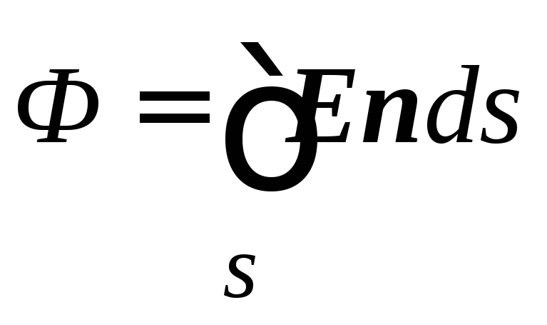
If the surface is closed, the flux of the tension vector is equal to
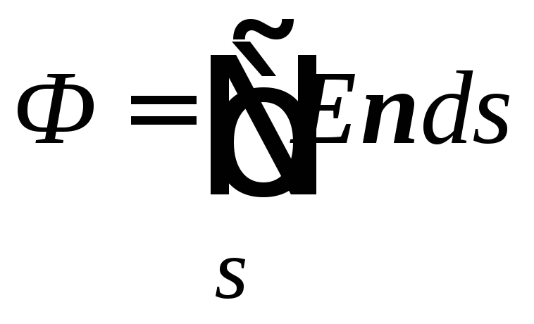 ,
,
i.e. the integral is taken over a closed surface s.
In this case, it is customary to direct the vector n outward from the surface. In this case, the flux through a closed surface is positive if the total charge covered by the closed surface is positive.
Dimension of the tension vector flow [F]=V. m=N. m 2 /Cl.
1.6. Gauss's theorem
Gauss's theorem is the fundamental theorem of electrostatics. It establishes a connection between the flow of the voltage vector through a closed surface and the total charge covered by this surface.
Let's consider this theorem.
Let the electric field be created by a positive point charge q.
Let us find the flow of the electric field strength vector through a closed surface enclosing this charge.
For the surface we choose a sphere of radius r, the center of which coincides with the charge q.
Since the charge creating the field is positive and located in the center of the sphere, the angle between the vector E and vector n is equal to zero at all points on the surface.
Therefore, the flow of the tension vector through the elementary surface ds will be equal En ds = E cos ds = E cos0 ds = Eds.
In other words, in the situation under consideration, the scalar product of the electrostatic field strength vector and the vector of the elementary surface is equal to the product of the moduli of these vectors.
The field strength created by a point charge is equal to 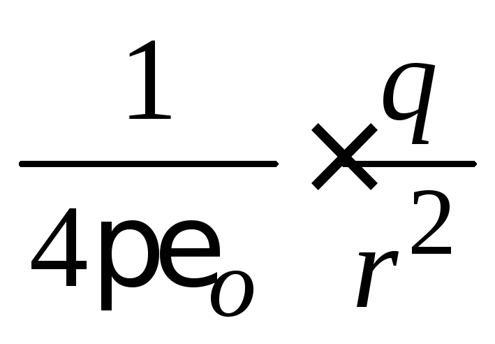 .
.
Since the charge is located in the center of the spherical surface, the distance from the charge to the surface at all its points is the same and equal r. Consequently, the modulus of the tension vector at all points of the spherical surface is the same: E= const.
The constant can be taken out of the integral sign, so the flux of the intensity vector through a closed surface in this case is equal to 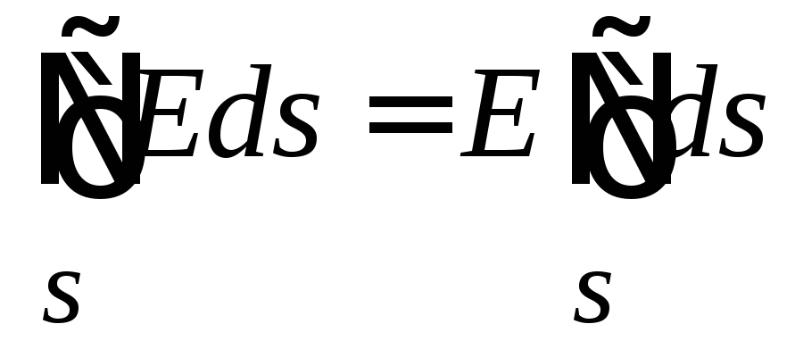 .
.
Integral of elementary surface areas s taken over the entire surface is equal to the area of this surface s. In this case, the surface is a sphere whose area s= 4 r 2 .
Thus, the flux of the tension vector through a closed surface in this case is equal to 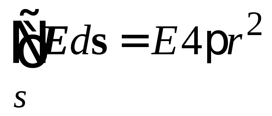 .
.
Substituting the expression for calculating the tension, we get
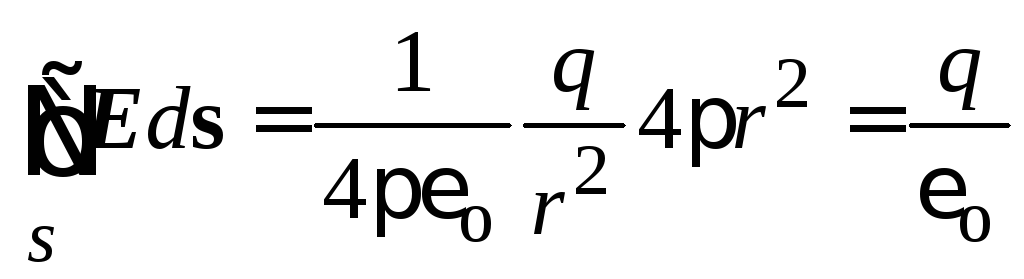 .
.
It can be shown that the flux of the field strength vector of a point charge through a closed surface will be equal to  and in the case when the charge is not in the center of the spherical surface.
Moreover, the flow will be the same even if the surface has any shape.
If the surface covers several charges q i, the flux of each charge through a closed surface will be equal to  . The total flux created by all charges will be equal to
  .
.
Changing the sequence of summation and integration and taking into account that, in accordance with the principle of superposition  , we get
 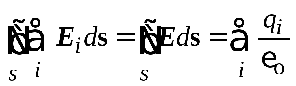 , Where E
– vector of the field strength created by all charges covered by a closed surface.
, Where E
– vector of the field strength created by all charges covered by a closed surface.
So, the analysis allowed us to obtain the following ratio:
 .
.
This relationship is universal in nature and is called Gauss’s theorem: the flow of the electric field strength vector through a closed surface is equal to the ratio of the sum of the charges covered by this surface to the electric constant.
Please note: in the expression of Gauss’s theorem there are no characteristics of the position of charges q i .
This means that the flow of the tension vector does not depend on how the charges covered by the closed surface are located. Moreover, the flux of the tension vector will not change if the relative arrangement of the charges covered by the surface changes.
The practical significance of Gauss's theorem is that it greatly simplifies the calculation of fields created by symmetrical charge distributions. In this case, you can choose a surface of such a shape that  , Where S
is the area of the part of the closed surface penetrated by the electric field.
, Where S
is the area of the part of the closed surface penetrated by the electric field.
E r =Ф S =4 2 =2 B m.
Example 2: a site S = 3m2 is located in a uniform field of 100 N/C. How many lines intersect this area if the angle is 30º (Fig. 2.4).
E ┴ = E sin 300 = 50 N/C
F = E ┴ · S = 50 · 3=150 lines
2.2. Tension vector flow.
So, using examples we have shown that if the field lines of a homogeneous
electric field with intensity E penetrate a certain area S, then the intensity flow (previously we called the number of field lines through the area) will be determined by the formula
Фr E = ES= EScos α= En S,
where E n is the product of the vector E and the normal to the given site (Fig. 2.5).

And the value F E here is called the flow of the electric field strength vector through the area S, i.e. definition:
The total number of lines of force passing through the surface S is called the flux of the FU intensity vector through this surface.
In vector form we can write
F E = (E,S) – scalar product of two vectors, |
|||
where vector S = n S. | |||
Those. vector flow |
|||
E is a scalar, which, depending on the angle α |
|||
can be both positive and negative . Let's consider (Fig. 2.6, 2.7).
For this configuration, the flux through surface A is negative (count the number of lines of force).
Rice. 2.6 Fig. 2.7
For Figure 2.6, surface A 1 is surrounded by a positive charge and the flow here is directed outward, i.e. Ф E > 0. Surface A 2 is surrounded by a negative charge and here Ф E< 0 направлен внутрь.
For Figure 2.7, the flux will not be zero if the total charge inside the surface is not zero. Those. flux depends on charge. This is the meaning of Gauss's theorem.
2.3. Ostrogradsky-Gauss theorem.
So, let’s remember the flow of the electric field strength vector – equal to the number tension lines passing through area S (Fig. 2.8).
dФЭ = EdScos α= En dS |
R2)
q 4 πR 2 = q
4 πε 0 R 2 2 2 ε 0
Those. in a uniform field F E =ES in an arbitrary electric field
FE = ∫ En dS= ∫ E dS | |||
d S r = dS n r – in vector form | |||
The orientation of dS in space is specified using the unit vector n r. Those. |
|||
– the direction coincides with the direction of the external normal to the surface. |
|||
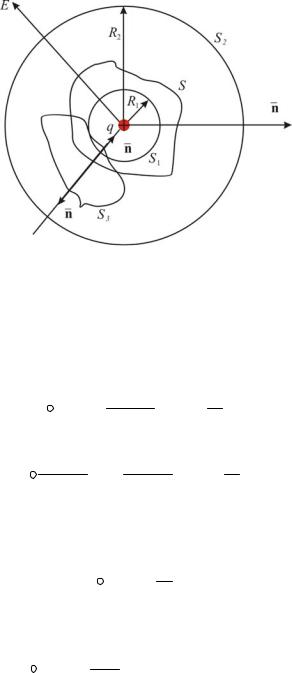
Let's calculate the flux of vector E through | closed surface | S surrounding |
|
point charge q (Fig. 2.9.).
The center of the circle coincides with the center of the charge. The radius of the sphere S 1 is equal to R 1 . IN
For each point of the surface S 1, the projection E to the direction of the external normal is the same and equal to
E n= | ||||||||
4πε | ||||||||
Then the flow through S 1 | ||||||||
ФE = ∫ En dS= | 2 4 πR 1 2 = | |||||||
4 πε0 R1 | ||||||||
Let's calculate the flow through S 2 (radius
FE = ∫ 4 πε q R 2 dS=
S 2 r 0 2
Lines of tension E begin and end at infinity) from the continuity of line E it follows that the flow of an arbitrary surface S will be equal to the same value:
FE = ∫ En dS= | |
The result obtained is valid not only for one charge, but also for any number of arbitrarily located charges located inside the surface
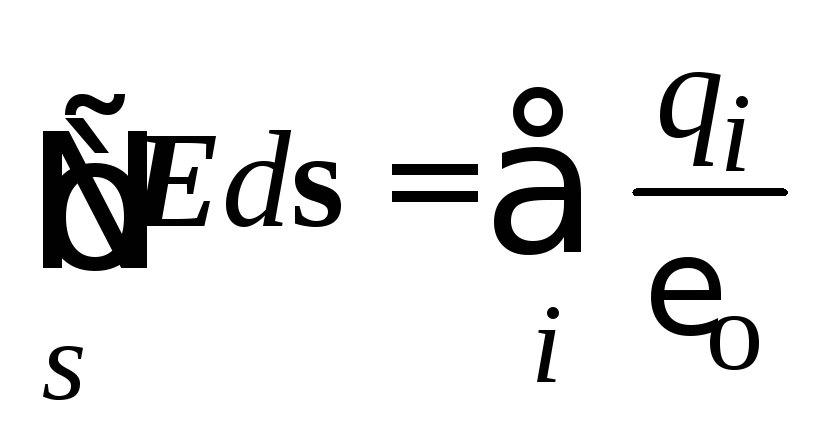
FE = ∫ En dS= | ∑q | – Gauss's theorem | ||
The flux of the electric field strength vector through a closed surface in vacuum is equal to the algebraic sum of all charges located inside the surface divided by ε0.
When calculating the flow through a closed surface, the normal vector n
limited by a given surface creates a positive flow, while the lines entering the volume create a negative flow.
If we place another surface S 3 between our spheres,
covering the charge, as can be seen from (Fig. 2.9). Each tension line E will cross this surface twice: once on the positive side - it will enter
into the surface S 3 , another time - from the negative side - it will come out of the surface S 3 .
IN the result is an algebraic sum of tension lines passing through
closed surface S 3 will be equal to zero, i.e. the total flux passing through S 3 is zero.
Thus, for a point charge q, the total flux through any closed surface S will be equal to:
FE = 0 – if the charge is located outside the closed surface and this result
does not depend on the shape of the surface and the sign of the flux coincides with the sign of the charge.
In the general case, electric charges can be “smeared” with a certain volumetric density ρ that varies in different places in space. Let's remember another concept - volumetric charge density
ρ = | |||||
where dV is the infinitesimal volume.
A physically infinitesimal volume dV should be understood as a volume that, on the one hand, is small enough so that within its limits the charge density can be considered the same, and on the other hand, large enough so that charge discreteness cannot appear, i.e. that any charge is a multiple of an integer number of elementary charges or P + (proton). Then the total charge
∑ qi = ∫ ρdV | |||
Then from Gauss’s theorem (2.3.7.) we write | |||
ε 0V ∫ | |||
This is another form of writing Gauss's theorem if the charge is continuous.
It is necessary to pay attention to the following circumstance: while r
the field E itself depends on the configuration of all charges, the flow E through an arbitrary closed surface is determined only by the algebraic sum of charges inside the surface S. This means that if you move the charges, then E will change everywhere, including on the surface S, but the flow of the vector E through this surface will remain the same. An amazing property of the tension vector E.
2.4. Differential form of Gauss's theorem.
IN It established a connection between the volumetric charge densityρ and change in E in the vicinity of a given point in space