The online calculator finds a solution to the system linear equations(SLN) using the Cramer method. Given detailed solution. To calculate, select the number of variables. Then enter the data into the cells and click on the "Calculate" button.
×
Warning
Clear all cells?
Close Clear
Data entry instructions. Numbers are entered as integers (examples: 487, 5, -7623, etc.), decimals (ex. 67., 102.54, etc.) or fractions. The fraction must be entered in the form a/b, where a and b (b>0) are integers or decimal numbers. Examples 45/5, 6.6/76.4, -7/6.7, etc.
Cramer method
The Cramer method is a method for solving a quadratic system of linear equations with a nonzero determinant of the main matrix. Such a system of linear equations has a unique solution.
Let the following system of linear equations be given:
Where A-main matrix of the system:
the first of which needs to be found, and the second is given.
Since we assume that the determinant Δ of the matrix A is different from zero, then there is an inverse to A matrix A-1 . Then multiplying identity (2) from the left by the inverse matrix A-1 , we get:
The inverse matrix has the following form:
Algorithm for solving a system of linear equations using the Cramer method
- Calculate the determinant Δ of the main matrix A.
- Replacing column 1 of a matrix A to the vector of free members b.
- Calculation of the determinant Δ 1 of the resulting matrix A 1 .
- Calculate Variable x 1 =Δ 1 /Δ.
- Repeat steps 2−4 for columns 2, 3, ..., n matrices A.
Examples of solving SLEs using Cramer's method
Example 1. Solve the following system of linear equations using the Cramer method:
Let's replace column 1 of the matrix A per column vector b:
Replace column 2 of the matrix A per column vector b:
Replace column 3 of the matrix A per column vector b:
The solution to a system of linear equations is calculated as follows:
Let's write it in matrix form: Ax=b, Where
We select the largest modulo leading element of column 2. To do this, we swap rows 2 and 4. In this case, the sign of the determinant changes to “−”.
We select the leading element of column 3, largest in modulus. To do this, we swap rows 3 and 4. In this case, the sign of the determinant changes to “+”.
We have reduced the matrix to upper triangular form. The determinant of the matrix is equal to the product of all elements of the main diagonal:
To calculate the determinant of a matrix A 1, we reduce the matrix to upper triangular form, similar to the above procedure. We get the following matrix:
Replace column 2 of the matrix A per column vector b, we reduce the matrix to upper triangular form and calculate the determinant of the matrix:
| ,,,. |
Let the system of linear equations contain as many equations as the number of independent variables, i.e. looks like
Such systems of linear equations are called quadratic. A determinant composed of coefficients for independent system variables(1.5) is called the main determinant of the system. We will denote it Greek letter D. So
If the main determinant contains an arbitrary ( j th) column, replace with a column of free terms of system (1.5), then you can get n auxiliary qualifiers:
(j = 1, 2, …, n). (1.7)
Cramer's rule solving quadratic systems of linear equations is as follows. If the main determinant D of system (1.5) is different from zero, then the system has a unique solution, which can be found using the formulas:
Example 1.5. Solve the system of equations using Cramer's method
Let us calculate the main determinant of the system:
Since D¹0, the system has a unique solution, which can be found using formulas (1.8):
Thus,
Actions on matrices
1. Multiplying a matrix by a number. The operation of multiplying a matrix by a number is defined as follows.
2. In order to multiply a matrix by a number, you need to multiply all its elements by this number. That is
Example 1.6. .
Matrix addition.
This operation is introduced only for matrices of the same order.
In order to add two matrices, it is necessary to add the corresponding elements of another matrix to the elements of one matrix:
(1.10)
The operation of matrix addition has the properties of associativity and commutativity.
Example 1.7. .
Matrix multiplication.
If the number of matrix columns A coincides with the number of matrix rows IN, then for such matrices the multiplication operation is introduced:
Thus, when multiplying a matrix A dimensions m´ n to the matrix IN dimensions n´ k we get a matrix WITH dimensions m´ k. In this case, the matrix elements WITH are calculated using the following formulas:
Problem 1.8. Find, if possible, the product of matrices AB And B.A.:
Solution. 1) In order to find a work AB, you need matrix rows A multiply by matrix columns B:
2) Work B.A. does not exist, because the number of matrix columns B does not match the number of matrix rows A.
Inverse matrix. Solving systems of linear equations using the matrix method
Matrix A- 1 is called the inverse of a square matrix A, if the equality is satisfied:
where through I denotes the identity matrix of the same order as the matrix A:
In order for a square matrix to have an inverse, it is necessary and sufficient that its determinant be different from zero. The inverse matrix is found using the formula:
Where A ij - algebraic additions to elements a ij matrices A(note that algebraic additions to matrix rows A are located in the inverse matrix in the form of corresponding columns).
Example 1.9. Find the inverse matrix A- 1 to matrix
We find the inverse matrix using formula (1.13), which for the case n= 3 has the form:
Let's find det A = | A| = 1 × 3 × 8 + 2 × 5 × 3 + 2 × 4 × 3 - 3 × 3 × 3 - 1 × 5 × 4 - 2 × 2 × 8 = 24 + 30 + 24 - 27 - 20 - 32 = - 1. Since the determinant of the original matrix is nonzero, the inverse matrix exists.
1) Find algebraic complements A ij:
For ease of location inverse matrix, we placed the algebraic additions to the rows of the original matrix in the corresponding columns.
From the obtained algebraic additions we compose a new matrix and divide it by the determinant det A. Thus, we get the inverse matrix:
Quadratic systems of linear equations with a nonzero principal determinant can be solved using the inverse matrix. To do this, system (1.5) is written in matrix form:
Multiplying both sides of equality (1.14) from the left by A- 1, we get the solution to the system:
Thus, in order to find a solution to a square system, you need to find the inverse matrix of the main matrix of the system and multiply it on the right by the column matrix of free terms.
Problem 1.10. Solve a system of linear equations
using the inverse matrix.
Solution. Let us write the system in matrix form: ,
where is the main matrix of the system, is the column of unknowns, and is the column of free terms. Since the main determinant of the system is , the main matrix of the system is A has an inverse matrix A-1 . To find the inverse matrix A-1 , we calculate the algebraic complements to all elements of the matrix A:
From the obtained numbers we will compose a matrix (and algebraic additions to the rows of the matrix A write it in the appropriate columns) and divide it by the determinant D. Thus, we have found the inverse matrix:
We find the solution to the system using formula (1.15):
Thus,
Solving systems of linear equations using the ordinary Jordan elimination method
Let an arbitrary (not necessarily quadratic) system of linear equations be given:
It is required to find a solution to the system, i.e. such a set of variables that satisfies all the equalities of system (1.16). In the general case, system (1.16) can have not only one solution, but also countless solutions. It may also have no solutions at all.
When solving such problems, the well-known school course method of eliminating unknowns is used, which is also called the ordinary Jordan elimination method. The essence this method lies in the fact that in one of the equations of system (1.16) one of the variables is expressed in terms of other variables. This variable is then substituted into other equations in the system. The result is a system containing one equation and one variable less than the original system. The equation from which the variable was expressed is remembered.
This process is repeated until one last equation remains in the system. Through the process of eliminating unknowns, some equations may become true identities, e.g. Such equations are excluded from the system, since they are satisfied for any values of the variables and, therefore, do not affect the solution of the system. If, in the process of eliminating unknowns, at least one equation becomes an equality that cannot be satisfied for any values of the variables (for example), then we conclude that the system has no solution.
If no contradictory equations arise during the solution, then one of the remaining variables in it is found from the last equation. If there is only one variable left in the last equation, then it is expressed as a number. If other variables remain in the last equation, then they are considered parameters, and the variable expressed through them will be a function of these parameters. Then the so-called “ reverse stroke" The found variable is substituted into the last remembered equation and the second variable is found. Then the two found variables are substituted into the penultimate memorized equation and the third variable is found, and so on, up to the first memorized equation.
As a result, we obtain a solution to the system. This solution will be unique if the found variables are numbers. If the first variable found, and then all the others, depend on the parameters, then the system will have an infinite number of solutions (each set of parameters corresponds to a new solution). Formulas that allow you to find a solution to a system depending on a particular set of parameters are called the general solution of the system.
Example 1.11.
x
After memorizing the first equation and bringing similar terms in the second and third equations, we arrive at the system:
Let's express y from the second equation and substitute it into the first equation:
Let us remember the second equation, and from the first we find z:
Working backwards, we consistently find y And z. To do this, we first substitute into the last remembered equation, from where we find y:
Then we substitute into the first remembered equation, from where we find x:
Problem 1.12. Solve a system of linear equations by eliminating unknowns:
Solution. Let us express the variable from the first equation x and substitute it into the second and third equations:
In this system, the first and second equations contradict each other. Indeed, expressing y from the first equation and substituting it into the second equation, we obtain that 14 = 17. This equality does not hold for any values of the variables x, y, And z. Consequently, system (1.17) is inconsistent, i.e. has no solution.
We invite readers to check for themselves that the main determinant of the original system (1.17) equal to zero.
Let us consider a system that differs from system (1.17) by only one free term.
Problem 1.13. Solve a system of linear equations by eliminating unknowns:
Solution. As before, we express the variable from the first equation x and substitute it into the second and third equations:
Let us remember the first equation and present similar terms in the second and third equations. We arrive at the system:
Expressing y from the first equation and substituting it into the second equation, we obtain the identity 14 = 14, which does not affect the solution of the system, and, therefore, it can be excluded from the system.
In the last remembered equality, the variable z we will consider it a parameter. We believe. Then
Let's substitute y And z into the first remembered equality and find x:
Thus, system (1.18) has an infinite number of solutions, and any solution can be found using formulas (1.19), choosing an arbitrary value of the parameter t:
(1.19)
So the solutions of the system, for example, are the following sets of variables (1; 2; 0), (2; 26; 14), etc. Formulas (1.19) express the general (any) solution of the system (1.18).
In the case when the original system (1.16) has sufficient a large number of equations and unknowns, the indicated method of ordinary Jordan elimination seems cumbersome. However, it is not. It is enough to derive an algorithm for recalculating the system coefficients at one step in general view and formulate the solution to the problem in the form of special Jordan tables.
Let a system of linear forms (equations) be given:
, (1.20)
Where x j- independent (sought) variables, a ij- constant coefficients
(i = 1, 2,…, m; j = 1, 2,…, n). Right parts of the system y i (i = 1, 2,…, m) can be either variables (dependent) or constants. It is required to find solutions to this system by eliminating the unknowns.
Let us consider the following operation, henceforth called “one step of ordinary Jordan eliminations”. From arbitrary ( r th) equality we express an arbitrary variable ( xs) and substitute into all other equalities. Of course, this is only possible if a rs¹ 0. Coefficient a rs called the resolving (sometimes guiding or main) element.
We will get the following system:
From s- equality of system (1.21), we subsequently find the variable xs(after the remaining variables have been found). S The -th line is remembered and subsequently excluded from the system. The remaining system will contain one equation and one less independent variable than the original system.
Let us calculate the coefficients of the resulting system (1.21) through the coefficients of the original system (1.20). Let's start with r th equation, which after expressing the variable xs through the remaining variables it will look like this:
Thus, the new coefficients r th equations are calculated using the following formulas:
(1.23)
Let us now calculate the new coefficients b ij(i¹ r) arbitrary equation. To do this, let us substitute the variable expressed in (1.22) xs V i th equation of system (1.20):
After bringing similar terms, we get:
(1.24)
From equality (1.24) we obtain formulas by which the remaining coefficients of system (1.21) are calculated (with the exception r th equation):
(1.25)
The transformation of systems of linear equations by the method of ordinary Jordan elimination is presented in the form of tables (matrices). These tables are called “Jordan tables”.
Thus, problem (1.20) is associated with the following Jordan table:
Table 1.1
| x 1 | x 2 | … | x j | … | xs | … | x n | |
| y 1 = | a 11 | a 12 | a 1j | a 1s | a 1n | |||
| ………………………………………………………………….. | ||||||||
| y i= | a i 1 | a i 2 | a ij | a is | a in | |||
| ………………………………………………………………….. | ||||||||
| y r= | a r 1 | a r 2 | a rj | a rs | arn | |||
| …………………………………………………………………. | ||||||||
| y n= | a m 1 | a m 2 | a mj | a ms | a mn |
Jordan table 1.1 contains a left header column in which the right parts of the system (1.20) are written and an upper header row in which independent variables are written.
The remaining elements of the table form the main matrix of coefficients of system (1.20). If you multiply the matrix A to the matrix consisting of the elements of the top title row, you get a matrix consisting of the elements of the left title column. That is, essentially, the Jordan table is a matrix form of writing a system of linear equations: . System (1.21) corresponds to the following Jordan table:
Table 1.2
| x 1 | x 2 | … | x j | … | y r | … | x n | |
| y 1 = | b 11 | b 12 | b 1 j | b 1 s | b 1 n | |||
| ………………………………………………………………….. | ||||||||
| y i = | b i 1 | b i 2 | b ij | b is | b in | |||
| ………………………………………………………………….. | ||||||||
| x s = | b r 1 | b r 2 | b rj | b rs | brn | |||
| …………………………………………………………………. | ||||||||
| y n = | b m 1 | b m 2 | b mj | bms | b mn |
Permissive element a rs We will highlight them in bold. Recall that to implement one step of Jordan elimination, the resolving element must be non-zero. The table row containing the enabling element is called the enabling row. The column containing the enable element is called the enable column. When moving from a given table to the next table, one variable ( xs) from the top header row of the table is moved to the left header column and, conversely, one of the free members of the system ( y r) moves from the left head column of the table to the top head row.
Let us describe the algorithm for recalculating the coefficients when moving from the Jordan table (1.1) to the table (1.2), which follows from formulas (1.23) and (1.25).
1. The resolving element is replaced by the inverse number:
2. The remaining elements of the resolving string are divided into the resolving element and change the sign to the opposite:
3. The remaining elements of the resolution column are divided into the resolution element:
4. Elements that are not included in the allowing row and allowing column are recalculated using the formulas:
The last formula is easy to remember if you notice that the elements that make up the fraction are at the intersection i-oh and r th lines and j th and s th columns (resolving row, resolving column, and the row and column at the intersection of which the recalculated element is located). More precisely, when memorizing the formula, you can use the following diagram:
When performing the first step of Jordan exceptions, you can select any element of Table 1.3 located in the columns as a resolving element x 1 ,…, x 5 (all specified elements are not zero). Just don't select the enabling element in the last column, because you need to find independent variables x 1 ,…, x 5 . For example, we choose the coefficient 1 with variable x 3 in the third line of Table 1.3 (the enabling element is shown in bold). When moving to table 1.4, the variable x The 3 from the top header row is swapped with the constant 0 of the left header column (third row). In this case, the variable x 3 is expressed through the remaining variables.
String x 3 (Table 1.4) can, after remembering in advance, be excluded from Table 1.4. The third column with a zero in the top title line is also excluded from Table 1.4. The point is that regardless of the coefficients of a given column b i 3 all corresponding terms of each equation 0 b i 3 systems will be equal to zero. Therefore, these coefficients need not be calculated. Eliminating one variable x 3 and remembering one of the equations, we arrive at a system corresponding to Table 1.4 (with the line crossed out x 3). Selecting in table 1.4 as a resolving element b 14 = -5, go to table 1.5. In Table 1.5, remember the first row and exclude it from the table along with the fourth column (with a zero at the top).
Table 1.5 Table 1.6
From the last table 1.7 we find: x 1 = - 3 + 2x 5 .
Consistently substituting the already found variables into the remembered lines, we find the remaining variables:
Thus, the system has infinitely many solutions. Variable x 5, arbitrary values can be assigned. This variable acts as a parameter x 5 = t. We proved the compatibility of the system and found it common decision:
x 1 = - 3 + 2t
x 2 = - 1 - 3t
x 3 = - 2 + 4t . (1.27)
x 4 = 4 + 5t
x 5 = t
Giving parameter t different values, we will obtain an infinite number of solutions to the original system. So, for example, the solution to the system is the following set of variables (- 3; - 1; - 2; 4; 0).
Cramer's method or the so-called Cramer's rule is a method of searching for unknown quantities from systems of equations. It can be used only if the number of sought values is equivalent to the number of algebraic equations in the system, that is, the main matrix formed from the system must be square and not contain zero rows, and also if its determinant must not be zero.
Theorem 1
Cramer's theorem If the main determinant $D$ of the main matrix, compiled on the basis of the coefficients of the equations, is not equal to zero, then the system of equations is consistent, and it has a unique solution. The solution to such a system is calculated through the so-called Cramer formulas for solving systems of linear equations: $x_i = \frac(D_i)(D)$
What is the Cramer method?
The essence of Cramer's method is as follows:
- To find a solution to the system using Cramer's method, first of all we calculate the main determinant of the matrix $D$. When the calculated determinant of the main matrix, when calculated by Cramer's method, turns out to be equal to zero, then the system does not have a single solution or has an infinite number of solutions. In this case, to find a general or some basic answer for the system, it is recommended to use the Gaussian method.
- Then you need to replace the outermost column of the main matrix with a column of free terms and calculate the determinant $D_1$.
- Repeat the same for all columns, obtaining determinants from $D_1$ to $D_n$, where $n$ is the number of the rightmost column.
- After all determinants $D_1$...$D_n$ have been found, the unknown variables can be calculated using the formula $x_i = \frac(D_i)(D)$.
Techniques for calculating the determinant of a matrix
To calculate the determinant of a matrix with a dimension greater than 2 by 2, you can use several methods:
- The rule of triangles, or Sarrus's rule, reminiscent of the same rule. The essence of the triangle method is that when calculating the determinant, the products of all numbers connected in the figure by the red line on the right are written with a plus sign, and all numbers connected in a similar way in the figure on the left are written with a minus sign. Both rules are suitable for matrices of size 3 x 3. In the case of the Sarrus rule, the matrix itself is first rewritten, and next to it its first and second columns are rewritten again. Diagonals are drawn through the matrix and these additional columns; matrix members lying on the main diagonal or parallel to it are written with a plus sign, and elements lying on or parallel to the secondary diagonal are written with a minus sign.
Figure 1. Triangle rule for calculating the determinant for Cramer's method
- Using a method known as the Gaussian method, this method is also sometimes called reducing the order of the determinant. In this case, the matrix is transformed and reduced to triangular form, and then all the numbers on the main diagonal are multiplied. It should be remembered that when searching for a determinant in this way, you cannot multiply or divide rows or columns by numbers without taking them out as a multiplier or divisor. In the case of searching for a determinant, it is only possible to subtract and add rows and columns to each other, having previously multiplied the subtracted row by a non-zero factor. Also, whenever you rearrange the rows or columns of the matrix, you should remember the need to change the final sign of the matrix.
- When solving a SLAE with 4 unknowns using the Cramer method, it is best to use the Gauss method to search and find determinants or determine the determinant by searching for minors.
Solving systems of equations using Cramer's method
Let's apply Cramer's method for a system of 2 equations and two required quantities:
$\begin(cases) a_1x_1 + a_2x_2 = b_1 \\ a_3x_1 + a_4x_2 = b_2 \\ \end(cases)$
Let's display it in expanded form for convenience:
$A = \begin(array)(cc|c) a_1 & a_2 & b_1 \\ a_3 & a_4 & b_1 \\ \end(array)$
Let's find the determinant of the main matrix, also called the main determinant of the system:
$D = \begin(array)(|cc|) a_1 & a_2 \\ a_3 & a_4 \\ \end(array) = a_1 \cdot a_4 – a_3 \cdot a_2$
If the main determinant is not equal to zero, then to solve the slough using Cramer’s method it is necessary to calculate a couple more determinants from two matrices with the columns of the main matrix replaced by a row of free terms:
$D_1 = \begin(array)(|cc|) b_1 & a_2 \\ b_2 & a_4 \\ \end(array) = b_1 \cdot a_4 – b_2 \cdot a_4$
$D_2 = \begin(array)(|cc|) a_1 & b_1 \\ a_3 & b_2 \\ \end(array) = a_1 \cdot b_2 – a_3 \cdot b_1$
Now let's find the unknowns $x_1$ and $x_2$:
$x_1 = \frac (D_1)(D)$
$x_2 = \frac (D_2)(D)$
Example 1
Cramer's method for solving SLAEs with a main matrix of 3rd order (3 x 3) and three required ones.
Solve the system of equations:
$\begin(cases) 3x_1 – 2x_2 + 4x_3 = 21 \\ 3x_1 +4x_2 + 2x_3 = 9\\ 2x_1 – x_2 - x_3 = 10 \\ \end(cases)$
Let's calculate the main determinant of the matrix using the rule stated above under point number 1:
$D = \begin(array)(|ccc|) 3 & -2 & 4 \\3 & 4 & -2 \\ 2 & -1 & 1 \\ \end(array) = 3 \cdot 4 \cdot ( -1) + 2 \cdot (-2) \cdot 2 + 4 \cdot 3 \cdot (-1) – 4 \cdot 4 \cdot 2 – 3 \cdot (-2) \cdot (-1) - (- 1) \cdot 2 \cdot 3 = - 12 – 8 -12 -32 – 6 + 6 = - 64$
And now three other determinants:
$D_1 = \begin(array)(|ccc|) 21 & 2 & 4 \\ 9 & 4 & 2 \\ 10 & 1 & 1 \\ \end(array) = 21 \cdot 4 \cdot 1 + (- 2) \cdot 2 \cdot 10 + 9 \cdot (-1) \cdot 4 – 4 \cdot 4 \cdot 10 – 9 \cdot (-2) \cdot (-1) - (-1) \cdot 2 \ cdot 21 = - 84 – 40 – 36 – 160 – 18 + 42 = - $296
$D_2 = \begin(array)(|ccc|) 3 & 21 & 4 \\3 & 9 & 2 \\ 2 & 10 & 1 \\ \end(array) = 3 \cdot 9 \cdot (- 1) + 3 \cdot 10 \cdot 4 + 21 \cdot 2 \cdot 2 – 4 \cdot 9 \cdot 2 – 21 \cdot 3 \cdot (-1) – 2 \cdot 10 \cdot 3 = - 27 + 120 + 84 – 72 + 63 – 60 = $108
$D_3 = \begin(array)(|ccc|) 3 & -2 & 21 \\ 3 & 4 & 9 \\ 2 & 1 & 10 \\ \end(array) = 3 \cdot 4 \cdot 10 + 3 \cdot (-1) \cdot 21 + (-2) \cdot 9 \cdot 2 – 21 \cdot 4 \cdot 2 - (-2) \cdot 3 \cdot 10 - (-1) \cdot 9 \cdot 3 = 120 – 63 – 36 – 168 + 60 + 27 = - $60
Let's find the required quantities:
$x_1 = \frac(D_1) (D) = \frac(- 296)(-64) = 4 \frac(5)(8)$
$x_2 = \frac(D_1) (D) = \frac(108) (-64) = - 1 \frac (11) (16)$
$x_3 = \frac(D_1) (D) = \frac(-60) (-64) = \frac (15) (16)$
Consider a system of 3 equations with three unknowns
Using 3rd order determinants, the solution to such a system can be written in the same form as for a system of two equations, i.e.
 (2.4)
(2.4)
if 0. Here
It's there Cramer's rule solving a system of three linear equations in three unknowns.
Example 2.3. Solve a system of linear equations using Cramer's rule:

Solution . Finding the determinant of the main matrix of the system

Since 0, then to find a solution to the system we can apply Cramer’s rule, but first we calculate three more determinants:

Examination:

Therefore, the solution was found correctly.
Cramer's rules derived for linear systems 2nd and 3rd order, suggest that the same rules can be formulated for linear systems of any order. Really happens
Cramer's theorem. Quadratic system of linear equations with a nonzero determinant of the main matrix of the system (0) has one and only one solution and this solution is calculated using the formulas
 (2.5)
(2.5)
Where – determinant of the main matrix, i – matrix determinant, obtained from the main one, replacingith column column of free members.
Note that if =0, then Cramer’s rule does not apply. This means that the system either has no solutions at all or has infinitely many solutions.
Having formulated Cramer's theorem, the question naturally arises of calculating determinants of higher orders.
2.4. Determinants of nth order
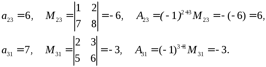
Additional minor M ij element a ij is a determinant obtained from a given by deleting i th line and j th column. Algebraic complement A ij element a ij the minor of this element taken with the sign (–1) is called i + j, i.e. A ij = (–1) i + j M ij .
For example, let's find the minors and algebraic complements of the elements a 23 and a 31 qualifiers

We get
Using the concept of algebraic complement we can formulate determinant expansion theoremn-th order by row or column.
Theorem 2.1. Matrix determinantAis equal to the sum of the products of all elements of a certain row (or column) by their algebraic complements:
 (2.6)
(2.6)
This theorem underlies one of the main methods for calculating determinants, the so-called. order reduction method. As a result of the expansion of the determinant n th order over any row or column, we get n determinants ( n–1)th order. To have fewer such determinants, it is advisable to select the row or column that has the most zeros. In practice, the expansion formula for the determinant is usually written as:

those. algebraic additions are written explicitly in terms of minors.
Examples 2.4. Calculate the determinants by first sorting them into some row or column. Typically, in such cases, select the column or row that has the most zeros. The selected row or column will be indicated by an arrow.


2.5. Basic properties of determinants
Expanding the determinant over any row or column, we get n determinants ( n–1)th order. Then each of these determinants ( n–1)th order can also be decomposed into a sum of determinants ( n–2)th order. Continuing this process, one can reach the 1st order determinants, i.e. to the elements of the matrix whose determinant is calculated. So, to calculate 2nd order determinants, you will have to calculate the sum of two terms, for 3rd order determinants - the sum of 6 terms, for 4th order determinants - 24 terms. The number of terms will increase sharply as the order of the determinant increases. This means that calculating determinants of very high orders becomes a rather labor-intensive task, beyond the capabilities of even a computer. However, determinants can be calculated in another way, using the properties of determinants.
Property 1 . The determinant will not change if the rows and columns in it are swapped, i.e. when transposing a matrix:
 .
.
This property indicates the equality of the rows and columns of the determinant. In other words, any statement about the columns of a determinant is also true for its rows and vice versa.
Property 2 . The determinant changes sign when two rows (columns) are interchanged.
Consequence . If the determinant has two identical rows (columns), then it is equal to zero.
Property 3 . The common factor of all elements in any row (column) can be taken out of the determinant sign.
For example,

Consequence . If all elements of a certain row (column) of a determinant are equal to zero, then the determinant itself is equal to zero.
Property 4 . The determinant will not change if the elements of one row (column) are added to the elements of another row (column), multiplied by any number.
For example,

Property 5 . The determinant of the product of matrices is equal to the product of the determinants of matrices:
Cramer's method is based on the use of determinants in solving systems of linear equations. This significantly speeds up the solution process.
Cramer's method can be used to solve a system of as many linear equations as there are unknowns in each equation. If the determinant of the system is not equal to zero, then Cramer’s method can be used in the solution, but if it is equal to zero, then it cannot. In addition, Cramer's method can be used to solve systems of linear equations that have a unique solution.
Definition. A determinant made up of coefficients for unknowns is called a determinant of the system and is denoted (delta).
Determinants
are obtained by replacing the coefficients of the corresponding unknowns with free terms:
 ;
;
 .
.
Cramer's theorem. If the determinant of the system is nonzero, then the system of linear equations has one unique solution, and the unknown is equal to the ratio of the determinants. The denominator contains the determinant of the system, and the numerator contains the determinant obtained from the determinant of the system by replacing the coefficients of this unknown with free terms. This theorem holds for a system of linear equations of any order.
Example 1. Solve a system of linear equations:
According to Cramer's theorem we have:

So, the solution to system (2):
online calculator, decisive method Kramer.
Three cases when solving systems of linear equations
As is clear from Cramer's theorem, when solving a system of linear equations, three cases can occur:

First case: a system of linear equations has a unique solution
(the system is consistent and definite)

Second case: a system of linear equations has an infinite number of solutions
(the system is consistent and uncertain)
** ![]() ,
,
those. the coefficients of the unknowns and the free terms are proportional.

Third case: the system of linear equations has no solutions
(the system is inconsistent)
So the system m linear equations with n called variables non-joint, if she does not have a single solution, and joint, if it has at least one solution. A simultaneous system of equations that has only one solution is called certain, and more than one – uncertain.
Examples of solving systems of linear equations using the Cramer method
Let the system be given
 .
.
Based on Cramer's theorem
………….
,
Where  -
-
system determinant. We obtain the remaining determinants by replacing the column with the coefficients of the corresponding variable (unknown) with free terms:


Example 2.
 .
.
Therefore, the system is definite. To find its solution, we calculate the determinants


Using Cramer's formulas we find:
![]()
So, (1; 0; -1) is the only solution to the system.
To check solutions to systems of equations 3 X 3 and 4 X 4, you can use an online calculator using Cramer's solving method.
If in a system of linear equations there are no variables in one or more equations, then in the determinant the corresponding elements are equal to zero! This is the next example.
Example 3. Solve a system of linear equations using the Cramer method:
 .
.
Solution. We find the determinant of the system:

Look carefully at the system of equations and at the determinant of the system and repeat the answer to the question in which cases one or more elements of the determinant are equal to zero. So, the determinant is not equal to zero, therefore the system is definite. To find its solution, we calculate the determinants for the unknowns


Using Cramer's formulas we find:
So, the solution to the system is (2; -1; 1).
To check solutions to systems of equations 3 X 3 and 4 X 4, you can use an online calculator using Cramer's solving method.
Top of page
We continue to solve systems using Cramer's method together
As already mentioned, if the determinant of the system is equal to zero, and the determinants of the unknowns are not equal to zero, the system is inconsistent, that is, it has no solutions. Let us illustrate with the following example.
Example 6. Solve a system of linear equations using the Cramer method:
Solution. We find the determinant of the system:
The determinant of the system is equal to zero, therefore, the system of linear equations is either inconsistent and definite, or inconsistent, that is, has no solutions. To clarify, we calculate determinants for unknowns

The determinants of the unknowns are not equal to zero, therefore, the system is inconsistent, that is, it has no solutions.
To check solutions to systems of equations 3 X 3 and 4 X 4, you can use an online calculator using Cramer's solving method.
In problems involving systems of linear equations, there are also those where, in addition to letters denoting variables, there are also other letters. These letters represent a number, most often real. In practice, search problems lead to such equations and systems of equations general properties any phenomena or objects. That is, have you invented any new material or a device, and to describe its properties, which are common regardless of the size or number of an instance, you need to solve a system of linear equations, where instead of some coefficients for variables there are letters. You don't have to look far for examples.
The following example is for a similar problem, only the number of equations, variables, and letters denoting a certain real number increases.
Example 8. Solve a system of linear equations using the Cramer method:

Solution. We find the determinant of the system:
Finding determinants for unknowns
